Data Processing

The Xplain software module designed for processing and interpretation the data obtained form microarrays images. The program works with files created by the Xplore image-processing module. Selecting the FileàOpen menu item opens the standard file open dialog.

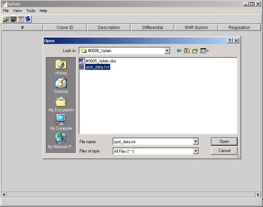
It is necessary to select the desired file with integral intensity data created by the Xplore module and press the <Open> button. The process of opening the file may take a few seconds because all the necessary calculations done by the program at this stage. After the file has opened the main window of the Xplain looks in the following way:

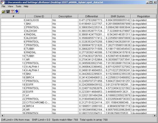
In the table that appeared as a result of opening the file each of the rows corresponds to the spot at the microarray. Meanings of the columns are following:

- # - serial number of a row in the table

- Clone ID - clone name the same that has been registered in the source microplate

- Description - non-mandatory description field transferred form the microplate registered

- Differential - value of the differential expression of the clone in the experiment

- SNR Summ - sum of SIGNAL to BACKGROUND ratios in the first and second scanning channels

- Regulation - positive differential represents an Up-regulated gene, negative is Down-regulated

Sorting.

By default the rows sorted by the differential descending. To sort them in the alphabetical order select the ToolsàFilter menu item and in the opened filter dialog

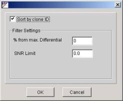
check the "Sort by clone ID" checkbox.

Calculations.

There are a number of parameters taken from the integral intensity file used for calculation of the differential expression of clones.

S1 - integral intensity of pixels from the SIGNAL area in the first scanning channel

S2 - integral intensity of pixels from the SIGNAL area in the second scanning channel

B1 - integral intensity of pixels from the BACKGROUND area in the first scanning channel

B2 - integral intensity of pixels from the BACKGROUND area in the second scanning channel

As - number of pixels in the SIGNAL area

Ab - number of pixels in the BACKGROUND area

Data Normalization.

Due to the difference in sensitivity of the scanners' channels and difference in the probes labeling a constant difference in the fluorescence level of the microarray surface in different channels may occur. This difference can be partially compensated by the normalization procedure:

The program calculates average signal of all spots on the microarrays in the firs and in the second channels:

Savg1 и Savg2.

The normalization coefficient is taken as a ratio of these values:

Knorm = Savg1/Savg2

Intensity of each spot in the second channel multiplies by this coefficient:

S1norm = S1

S2norm = S2 x Knorm

Differential Expression Calculation.

Differential = log( S1norm / S2norm )

Signal to Background Ratio Calculation.

The signal and the background areas may contain different amount of pixels. Due to this it is necessary to deal with the values of signal and background densities instead of dealing with direct values:

Ds1 = S1/As - signal density in the first channel

Ds2 = S2/As - signal density in the second channel

Db1 = B1/Ab - background density in the first channel

Db2 = B2/Ab - background density in the second channel

SNR summ = Ds1/Db1 + Ds2/Db2

All above calculations take place for each spot on the microarray.

Quality Control Data.

The Xplain presents data that helps making conclusions regarding quality of the experiment.

The ToolsàQC menu item opens the QC dialog window.

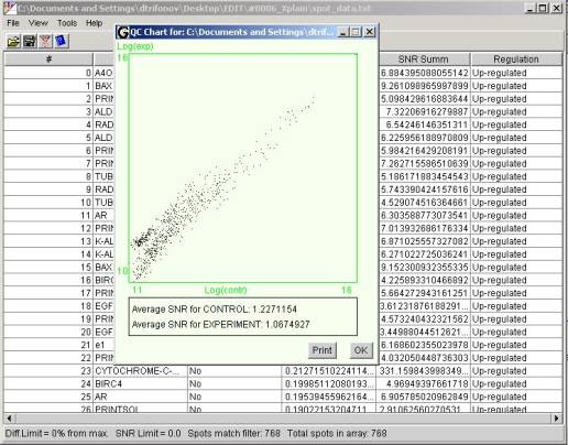
In the upper part of the window resides the scatter plot. Values along the X and Y axes are logarithms of normalized intensities in the first and in the second scanning channels correspondingly. Each spot on the microarray represented by a dot on the scatter plot.

It can be the following interpretation to the scatter plot. Most of the spots at a reasonably large microarray have close to zero differentials. Therefore ideally most of the scatter plot dots suppose to be concentrated along the diagonal line coming from the left lower corner of the chart area. All deviations of spots from the diagonal can be caused either by the differential expression or by an error in the experiment. If most of the spots scattered away from the diagonal that picture can be interpreted, as multiple errors exist in the experiment. In the particular example shown at the picture above scattering of the dots can be explained by a rather low signal to background ration of the whole experiment. Average values of the signal to background ratios for both channels shown under the chart area in the QC window. The fact that apparently most of the spots reside over the diagonal indicates that the numerical normalization of the data was not enough to correct the difference in the channels completely. It would be expedient to re-scan the microarray and do channels leveling based on the background integral intensity. This information can be obtained using the Xplore statistical analysis tools. Noticeable aggregation of spots in the left lower corner slightly apart from the rest of the spots can be caused buy a runs or drops of washing liquid dried on the microarray surface affecting it's uniformity.

For comparison there is a chart of a microarray data obtained from the high quality experiment and processed in a proper way. In spite of a very low signal to background ratio, around 3, the data has small dispersion and therefore high reliability and repeatability.

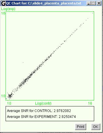
One spot placed significantly away from the rest of the spots conglomerate corresponds to a prelabeled control clone that supposed to have a large differential.

Data Selection.

Not all spots may be of interest to an experimenter. It makes sense to exclude from consideration all spots with too low signal to background ratio because they provide unreliable data. Signal to background credibility threshold differs from one experiment to another. It can be determined by comparing data from spots duplicates. And that is the reason to duplicate spots on the array whenever it's possible in order to have the comparison basis. It is known from the experience that in the most of experiments spots with the signal to background ratio over 5-6 give credible information.

In order to set the S/B threshold and let the program filter out all spots below that level select the ToolsàFilter menu item and in the opened filter dialog enter the desired value in the "SNR Limit" field.

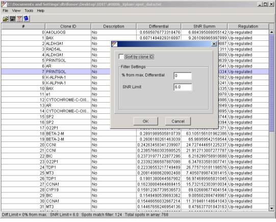
After that has done the table reflect only rows that match the filter criterion. The status bar at the Xplain main window shows how many spots have been selected. In this example for the S/N threshold equal to 6:

Spots match filter: 124-selected 124 spots

from

Total spots in array: 768.

Differential Expression Level Selection.

The second parameter of the filter defines the differential expression threshold in the percentage from the maximal differential expression found at a particular microarray. The 0 value of this parameter allows all spots to be shown, the 100 value results in selection of only one spot the one that has the highest differential expression level. The two filter parameters liked with the logical "AND" function therefore selected data must comply with both criteria of the filter.

In the example following filter settings:

% from max. Differential = 90

SNR limit = 6.0

will drop off all rows. It means that spots with the highest differential expression do not mach the S/N criterion and provide unreliable data.

Data Exporting.

The table data can be saved in a .TXT file for further processing by another applications. Use the FileàSave As menu item in order to do this.

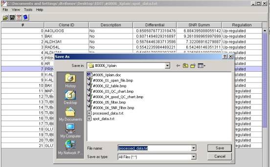
Only the rows that match filer criteria will be placed in the file. File structure is identical to the structure of the table. Columns separated by the " , " (comma) symbol.