

This user's guide describes the operation of the new version of Spectrum, and assumes that you are familiar with the basics of spectral analysis.
For the Macintosh versions (68K and PPC) there is very little installation necessary: simply extract the program applications and place them where you want on your hard disc. Since they come as binhex'd self-extracting archives, this will be automatic on most machines.
In order to correctly display trees in the log window, Spectrum uses a font called "COMPONENTMonaco." To use this font, drop the "COMPONENT Font File" onto your System folder.

 |
Spectrum can import both interleaved and sequential format PHYLIP files. However it cannot read files that have options such as "W" (weights). |
 |
Spectrum will read distance matrices in either lower-left, upper-right, or square formats. However, it will not handle replicates, or other options. |
In order to convert four-state characters to two-state characters you must specify a mapping. By default, Spectrum converts nucleotide data to purines and pyrimidines. You can change this using the Mapping command. This command displays the following dialog box:
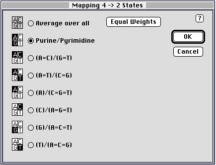
The Average over all option extracts splits by averaging over all the possible mappings, and allows you to specify the weights for each possible mapping. The default is to treat each mapping equally.
| Hamming | The proportion of sites at which the two sequences differ. |
| Jukes-Cantor | Assumes equal base frequencies and no transition/transversion bias. |
| Kimura 2-parameter | Assumes equal base frequencies and allows a transition/transversion bias. |
| Tamura-Nei | Allows for unequal base frequencies and a transition/transversion bias. Similar to the HKY85 model, but Tamura-Nei allows the two types of transition to occur at different frequencies. |
| LogDet | Designed to overcome the effects of unequal base composition. |
| Nucleotide composition | Not intended a measure of evolutionary distance, but simply how similar the sequences in their base composition. |
Once the distance matrix is calculated, a distance spectrum can be constructed. If the distances are additive, then the distance spectrum will contain the edge lengths of the underlying tree; if the distances deviate from additivity then there will be some other splits with positive support values.
 |
Rank the splits by their support, and display each split's conflict below that split. This is the default option |

|
Rank the splits by their support; conflicts are not shown. |
 |
The splits are plotted in the order of their split number, and display the conflict for each split. |

|
The splits are plotted in the order of their split number; conflicts are not shown. |
If you are going to display the split conflict values, you can choose to normalise the conflicts by the number of conflicting splits, or by the number of splits that could possibly conflict with that split.
If you chose the Plot command the program will display the spectrum in a separate chart window:
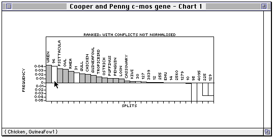
The splits are coloured light grey if they correspond to terminal taxa, and otherwise are white. If you have computed a tree then the splits in that tree will be coloured black. Pendant splits are labelled by the corresponding taxon name; internal splits are labelled by their split number.
 Hints
HintsYou can get the support and conflict of individual splits by using the Evaluate bipartition and Evaluate split commands. These do exactly the same thing, however the Evaluate split command requires you to know the number of the split you want to look at. If you don't know the number, you can use the Evaluate bipartition command, which displays the following dialog box:
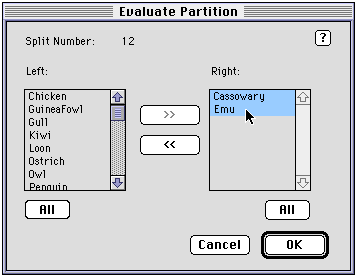
By moving taxa from the left-hand list to the right-hand list you create a split. The corresponding split number is displayed at the top of the dialog box. In this example the split {Cassowary, Emu} is shown, which is split 12.
Spectrum computes both closest (not yet) and Manhattan trees. Once you have a
tree you can display the tree in the log window using the Show tree and
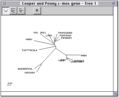
The toolbar at the top of the tree window has the following buttons to control how the tree is displayed.
 |
Display the tree as an unrooted tree. This is the default option |
 |
Display the tree as a rooted tree (cladogram). |
 |
Display the tree as a rooted tree with branch lengths proportional to split support. |
 |
Toggle on and off the display of the split number each edge in the tree corresponds to. |
This will display a chart of the support for each internal edge in the tree, and the two edges that correspond to the two nearest neighbour interchanges (NNI's) around that edge. In other words, you can see whether making a given edge is strongly supported relative to a local rearrangement of that tree.
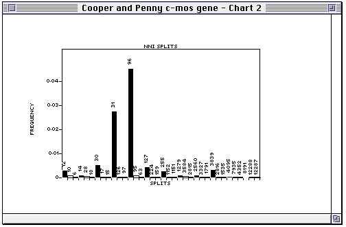
In the NNI plot, each internal edge in the tree is plotted, followed by the two NNI edges. For example, in the plot below

split 12 is in the tree, and splits 10 and 6 are the two splits we obtain by interchanging the nearest neighbours around split 12. In this example, there is rather less support for 10, and very little for 6. If either of the alternative splits had similar support to the split in the tree then that edge could be judged poorly supported.
You can also save your output for use by other programs. For example, a spectrum can be saved as a tab-delimited text file for importing into a spreadsheet program such as Excel. Any trees you have found can be saved as NEXUS tree files which can be viewed by TreeView, and read into programs that support NEXUS files such as PAUP and MacClade.
Spectrum can save your data to a NEXUS format file that has the following icon:

This file contains the following:
 Warning